GRASS GIS es el primer SIG de código abierto que incorporó capacidades para gestionar, analizar, procesar y visualizar datos espacio-temporales, así como las relaciones temporales entre series de tiempo.
Completamente basado en metadatos, por lo que no hay duplicación de datos
Sigue una aproximación Snapshot, i.e., añade marcas de tiempo o timestamps a los mapas
Una colección de mapas de la misma variable con timestamps se llama space-time dataset o STDS
Los mapas en una STDS pueden tener diferentes extensiones espaciales y temporales
TGRASS utiliza una base de datos SQLite para almacenar la extensión temporal y espacial de las STDS, así como las relaciones topológicas entre los mapas y entre las STDS en cada mapset.
TGRASS o GRASS GIS temporal framework fue desarrollado por Sören Gebbert como parte de un proyecto Google Summer of Code en 2012. Detalles técnicos de la implementación pueden encontrarse en: Gebbert y Pebesma (2014), Gebbert y Pebesma (2017) y Gebbert et al. (2019).
Space-time datasets
Space time raster datasets (STRDS)
Space time 3D raster datasets (STR3DS)
Space time vector datasets (STVDS)
Otras nociones básicas en TGRASS
El tiempo puede definirse como intervalos (inicio y fin) o como instancias (sólo inicio)
El tiempo puede ser absoluto (por ejemplo, 2017-04-06 22:39:49) o relativo (por ejemplo, 4 años, 90 días)
Granularidad es el mayor divisor común de todas las extensiones temporales (y posibles gaps) de los mapas de un STDS
Series de diferente granularidad y tipo de tiempo
Topología se refiere a las relaciones temporales entre los intervalos de tiempo en una STDS
Relaciones topológicas entre STDS y entre mapas
Muestreo temporal se utiliza para determinar el estado de un proceso respecto un segundo proceso.
Muestreo temporal
Módulos temporales
t.*: Módulos generales para manejar STDS de todos los tipos
t.rast.*: Módulos que tratan con STRDS
t.rast3d.*: Módulos que tratan con STR3DS
t.vect.*: Módulos que tratan con STVDS
TGRASS: marco general y flujo de trabajo
Manos a la obra
En esta segunda parte de la sesión vamos a recorrer los módulos temporales de GRASS GIS y demostrar su funcionalidad por medio de una serie de datos de temperatura de superficie (LST) de MODIS.
Antes de empezar y para ganar tiempo, conectamos nuestro drive e instalamos GRASS en Google Colab.
# import drive from google colabfrom google.colab import drive# mount drivedrive.mount("/content/drive")
import os# data directoryhomedir ="/content/drive/MyDrive/curso_grass_2023"# change to homedir so output files will be saved thereos.chdir(homedir)# GRASS GIS database variablesgrassdata = os.path.join(homedir, "grassdata")project ="posgar2007_4_cba"mapset ="modis_lst"
# import standard Python packages we needimport sysimport subprocess# ask GRASS GIS where its Python packages are to be able to run it from the notebooksys.path.append( subprocess.check_output(["grass", "--config", "python_path"], text=True).strip())
Importamos los paquetes de GRASS e iniciamos una sesión:
# import the GRASS GIS packages we needimport grass.script as gsimport grass.jupyter as gj# Start the GRASS GIS Sessionsession = gj.init(grassdata, project, mapset)
# show current GRASS GIS settings, this also checks if the session worksgs.gisenv()
Región computacional y máscara
Listar los mapas raster y obtener información de uno de ellos
# get list of raster maps in the 'modis_lst' mapsetlista_mapas = gs.list_grouped(type="raster")["modis_lst"]lista_mapas[:8]
# Get info from one of the raster mapsgs.raster_info(map="MOD11B3.A2015001.h12v12.single_LST_Day_6km")
Vamos a agregar el semantic label a cada mapa de LST
# list only LST mapslista_lst = gs.list_grouped(type="raster", pattern="*LST_Day*")["modis_lst"]
# set semantic labelsfor i in lista_lst: gs.run_command("r.support",map=i, semantic_label="LST")
# Get info from one of the raster mapsgs.raster_info(map="MOD11B3.A2015001.h12v12.single_LST_Day_6km")["semantic_label"]
Establecemos la región computacional
# set region to Cba boundaries with LST maps' resolutionprint(gs.read_command("g.region", vector="provincia_cba", align="MOD11B3.A2015001.h12v12.single_LST_Day_6km", flags="p"))
Aplicamos la máscara con los límites de la provincia de Córdoba
# set a MASK to Cba boundarygs.run_command("r.mask", vector="provincia_cba")
Crea una tabla SQLite en la base de datos temporal
Permite manejar grandes cantidades de mapas usando el STDS como entrada
Necesitamos especificar:
tipo de mapas (raster, raster3d o vector)
tipo de tiempo (absoluto o relativo)
Creamos la STRDS
# Create the STRDSgs.run_command("t.create",type="strds", temporaltype="absolute", output="LST_Day_monthly", title="Monthly LST Day 5.6 km", description="Monthly LST Day 5.6 km MOD11B3.006 Cordoba, 2015-2019")
Chequear si la STRDS fue creada
# Check if the STRDS is createdgs.read_command("t.list",type="strds")
Obtener información sobre la STRDS
# Get info about the STRDSprint(gs.read_command("t.info", input="LST_Day_monthly"))
Gráfico temporal de LST para la ciudad de Córdoba, Argentina
# LST time series plot for Cba city center!g.gui.tplot strds=LST_Day_monthly_celsius coordinates=4323478.531282977,6541664.09350761 title="Monthly LST. City center of Cordoba" xlabel="Time" ylabel="LST"
Salida de g.gui.tplot
En la interfaz de g.gui.tplot, las coordenadas del punto pueden ser escritas directamente, copiadas desde el mapa o seleccionadas interactivamente en el map display.
# Maps with minimum value lower than or equal to 10print(gs.read_command("t.rast.list",input="LST_Day_monthly_celsius", order="min", columns="name,start_time,min", where="min <= '10.0'"))
Mapas cuyo valor máximo es mayor a 30
# Maps with maximum value higher than 30print(gs.read_command("t.rast.list",input="LST_Day_monthly_celsius", order="max", columns="name,start_time,max", where="max > '30.0'"))
Mapas contenidos entre dos fechas
# Maps between two given datesprint(gs.read_command("t.rast.list",input="LST_Day_monthly_celsius", columns="name,start_time", where="start_time >= '2015-05' and start_time <= '2015-08-01 00:00:00'"))
Todos los mapas correspondientes al mes de Enero
# Maps from Januaryprint(gs.read_command("t.rast.list",input="LST_Day_monthly_celsius", columns="name,start_time", where="strftime('%m', start_time)='01'"))
Estadística descriptiva de STRDS
Imprimir estadísticas descriptivas univariadas para cada mapa dentro de la STRDS
# Print univariate stats for maps within STRDSprint(gs.read_command("t.rast.univar",input="LST_Day_monthly_celsius"))
Obtener estadísticas extendidas con la opción -e y escribir la salida a un archivo de texto
# Write extended univariate stats output to a csv filegs.run_command("t.rast.univar", flags="e",input="LST_Day_monthly_celsius", output=os.path.join(homedir,"ext_stats_LST_Day_monthly_celsius.csv"), separator="comma")
Graficamos las series del promedio, mínimo y máximo por mapa:
# Read the csv and plotimport pandas as pdlst = pd.read_csv(os.path.join(homedir,"ext_stats_LST_Day_monthly_celsius.csv"))lst['start'] = pd.to_datetime(lst.start, format="%Y-%m-%d", exact=False)lst.plot.line(1, [3,4,5], subplots=False)
Agrega STRDS completas o partes de ellas usando la opción where.
Diferentes métodos disponibles: promedio, mínimo, máximo, mediana, moda, etc.
LST máxima y mínima del período 2015-2019
Obtener los mapas de la máxima y mínima LST del período
# Get maximum and minimum LST in the STRDSmethods=["maximum","minimum"]for m in methods: gs.run_command("t.rast.series",input="LST_Day_monthly_celsius", output=f"LST_Day_{m}", method=m)
Cambiar la paleta de colores a celsius
# Change color pallete to celsiusgs.run_command("r.colors",map="LST_Day_minimum,LST_Day_maximum", color="celsius")
Usamos la calculadora de mapas temporal, t.rast.mapcalc,para obtener el mes de la LST mínima
# Get month of maximum LSTexpression="if(LST_Day_monthly_celsius == LST_Day_minimum, start_month(), null())"gs.run_command("t.rast.mapcalc", flags="n", inputs="LST_Day_monthly_celsius", output="month_min_lst", expression=expression, basename="month_min_lst")
Obtener información del mapa resultante
# Get basic infoprint(gs.read_command("t.info", input="month_min_lst"))
Obtenemos el primer mes en que aparece el mínimo de LST
# Get the earliest month in which the maximum appeared (method minimum)gs.run_command("t.rast.series",input="month_min_lst", method="minimum", output="min_lst_date")
Remover la STRDS intermedia y los mapas que contiene:
# Remove month_min_lst strds # we were only interested in the resulting aggregated mapgs.run_command("t.remove", flags="rfd", inputs="month_min_lst")
Chequeamos que la serie fue removida
# check STRDS in our mapsetprint(gs.read_command("t.list"))
Mostrar el mapa resultante con la clase Map de grass.jupyter
Podríamos haber hecho lo mismo pero anualmente para conocer en qué mes ocurre el máximo en cada año y así evaluar la ocurrencia de tendencias. Cómo lo harían?
Establecer la paleta de colores celsius para la STRDS estacional
# Set STRDS color table to celsius degreesgs.run_command("t.rast.colors",input="LST_Day_mean_3month", color="celsius")
Mostramos la serie recientemente creada con una animación. Para eso vamos a usar la clase TimeSeriesMap de grass.jupyter
## Display newly created NDVI time series maplstseries = gj.TimeSeriesMap(use_region=True)lstseries.add_raster_series("LST_Day_mean_3month", fill_gaps=False)lstseries.d_legend(color="black", at=(10,40,2,6))lstseries.show() # Create TimeSlider# optionally, write out to animated GIFlstseries.save("lstseries.gif")
Tarea
Ahora que ya conocen t.rast.aggregate, extraigan el mes de máximo LST por año y luego vean si hay alguna tendencia positiva o negativa, es decir, si los valores máximos de LST se observan más tarde o más temprano con el tiempo (años).
# January average LSTgs.run_command("t.rast.series",input="LST_Day_monthly_celsius", method="average", where="strftime('%m', start_time)='01'", output="LST_average_jan")
Climatología para todos los meses
# for all monthsmonths=['{0:02d}'.format(m) for m inrange(1,13)]methods=["average"]for m in months:for me in methods: gs.run_command("t.rast.series", input="LST_Day_monthly_celsius", method=me, where=f"strftime('%m', start_time)='{m}'", output=f"LST_{me}_{m}")
Tarea
Comparar las medias mensuales con las climatologías mensuales
Las climatologías que creamos forman una STRDS?
Anomalías anuales
Se necesitan:
promedio y desviación estándar general de la serie
promedios anuales
\[
AnomaliaStd_i = \frac{Media_i - Media}{SD}
\]
Obtenemos primero el promedio y el desvío estándar general de la serie
# Get general average and SDmethods=["average","stddev"]for me in methods: gs.run_command("t.rast.series",input="LST_Day_monthly_celsius", method=me, output=f"LST_Day_{me}")
y luego los promedios anuales
# Get annual averagesgs.run_command("t.rast.aggregate",input="LST_Day_monthly_celsius", method="average", granularity="1 years", output="LST_yearly_average", basename="LST_yearly_average")
Utilizamos el álgebra temporal para estimar las anomalías anuales
Remover el área del buffer 15 km del buffer de 30 km
# Remove 15km buffer area from the 30km buffer areags.run_command("v.overlay", ainput="cba_summer_lst_buf15", binput="cba_summer_lst_buf30", operator="xor", output="cba_surr")
Límites del Gran Córdoba y el área rural circundante
Extraer estadísticas para los alrededores del Gran Córdoba
# crear un data frame a partir del vectortabla2 = pd.DataFrame.from_dict(gs.vector_db_select(map="cba_surr_summer_lst")['values'], orient='index', columns=gs.vector_db_select(map="cba_surr_summer_lst")['columns'])tabla2
Gebbert, S., Leppelt, T., y Pebesma, E. (2019), «A TopologyBasedSpatio-TemporalMapAlgebra for BigDataAnalysis», Data, 4, 86. https://doi.org/10.3390/data4020086.
Gebbert, S., y Pebesma, E. (2014), «A temporal GIS for field based environmental modeling», Environmental Modelling & Software, 53, 1-12. https://doi.org/10.1016/j.envsoft.2013.11.001.
Gebbert, S., y Pebesma, E. (2017), «The GRASSGIS temporal framework», International Journal of Geographical Information Science, 31, 1273-1292. https://doi.org/10.1080/13658816.2017.1306862.
Ejecutar el código
---title: Intro a series de tiempoauthor: Verónica Andreodate: todayformat: html: code-tools: true code-copy: true code-fold: falseexecute: eval: false cache: false keep-ipynb: truejupyter: python3---# TGRASS: GRASS Temporal**GRASS GIS** es **el primer SIG de código abierto** que incorporó capacidades para **gestionar, analizar, procesar y visualizar datos espacio-temporales**,así como las relaciones temporales entre series de tiempo.- Completamente [basado en metadatos]{style="color: #18bc9c;"}, por lo que no hay duplicación de datos- Sigue una aproximación [*Snapshot*]{style="color: #18bc9c;"}, i.e., añade marcas de tiempo o *timestamps* a los mapas- Una colección de mapas de la misma variable con timestamps se llama [space-time dataset o STDS]{style="color: #18bc9c;"}- Los mapas en una STDS pueden tener diferentes extensiones espaciales y temporales- TGRASS utiliza una base de datos [SQLite](https://www.sqlite.org/index.html)para almacenar la extensión temporal y espacial de las STDS, así como las relaciones topológicas entre los mapas y entre las STDS en cada mapset.TGRASS o GRASS GIS temporal framework fue desarrollado por Sören Gebbert comoparte de un proyecto Google Summer of Code en 2012. Detalles técnicos de la implementación pueden encontrarse en: @gebbert_temporal_2014, @gebbert_grass_2017 y @gebbert_topology_2019.## Space-time datasets- Space time raster datasets ([**STRDS**]{style="color: #18bc9c;"})- Space time 3D raster datasets ([**STR3DS**]{style="color: #18bc9c;"})- Space time vector datasets ([**STVDS**]{style="color: #18bc9c;"})## Otras nociones básicas en TGRASS- El tiempo puede definirse como **intervalos** (inicio y fin) o como **instancias** (sólo inicio)- El tiempo puede ser **absoluto** (por ejemplo, 2017-04-06 22:39:49) o **relativo** (por ejemplo, 4 años, 90 días)- *Granularidad* es el mayor divisor común de todas las extensiones temporales(y posibles gaps) de los mapas de un STDS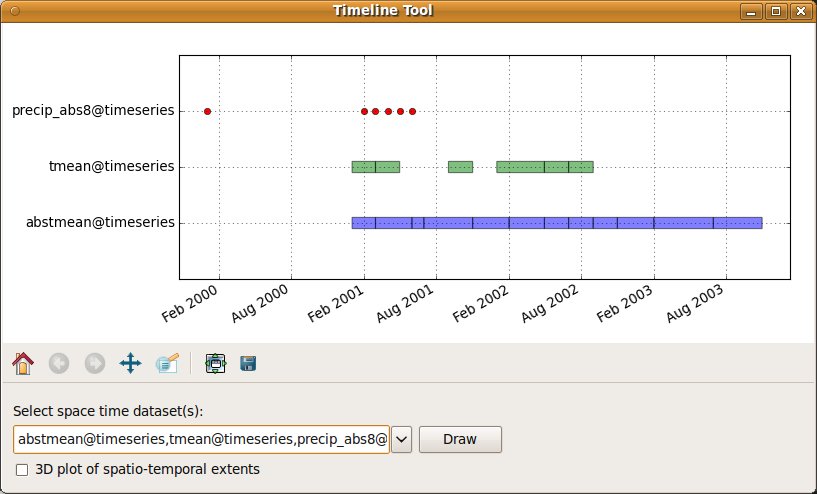{width="50%" fig-align="center"}- *Topología* se refiere a las relaciones temporales entre los intervalos de tiempo en una STDS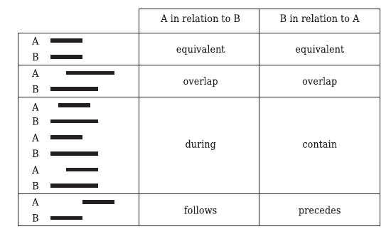{width=70%}- *Muestreo temporal* se utiliza para determinar el estado de un proceso respecto un segundo proceso.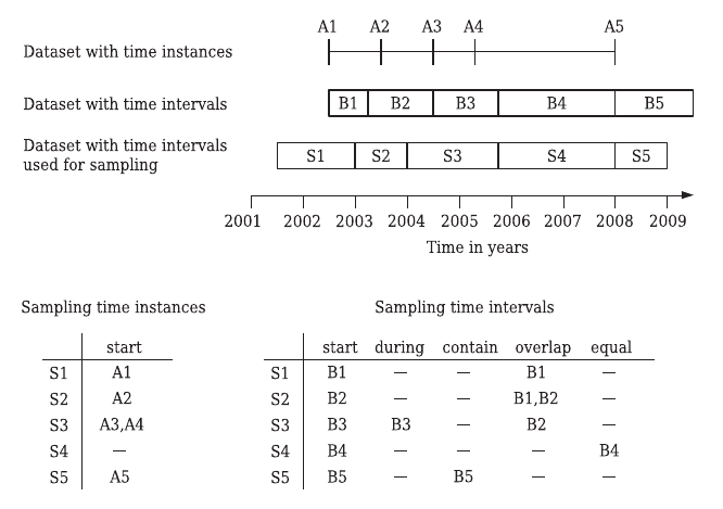{width=55%}## Módulos temporales- **t.\***: Módulos generales para manejar STDS de todos los tipos- **t.rast.\***: Módulos que tratan con STRDS- **t.rast3d.\***: Módulos que tratan con STR3DS- **t.vect.\***: Módulos que tratan con STVDS## TGRASS: marco general y flujo de trabajo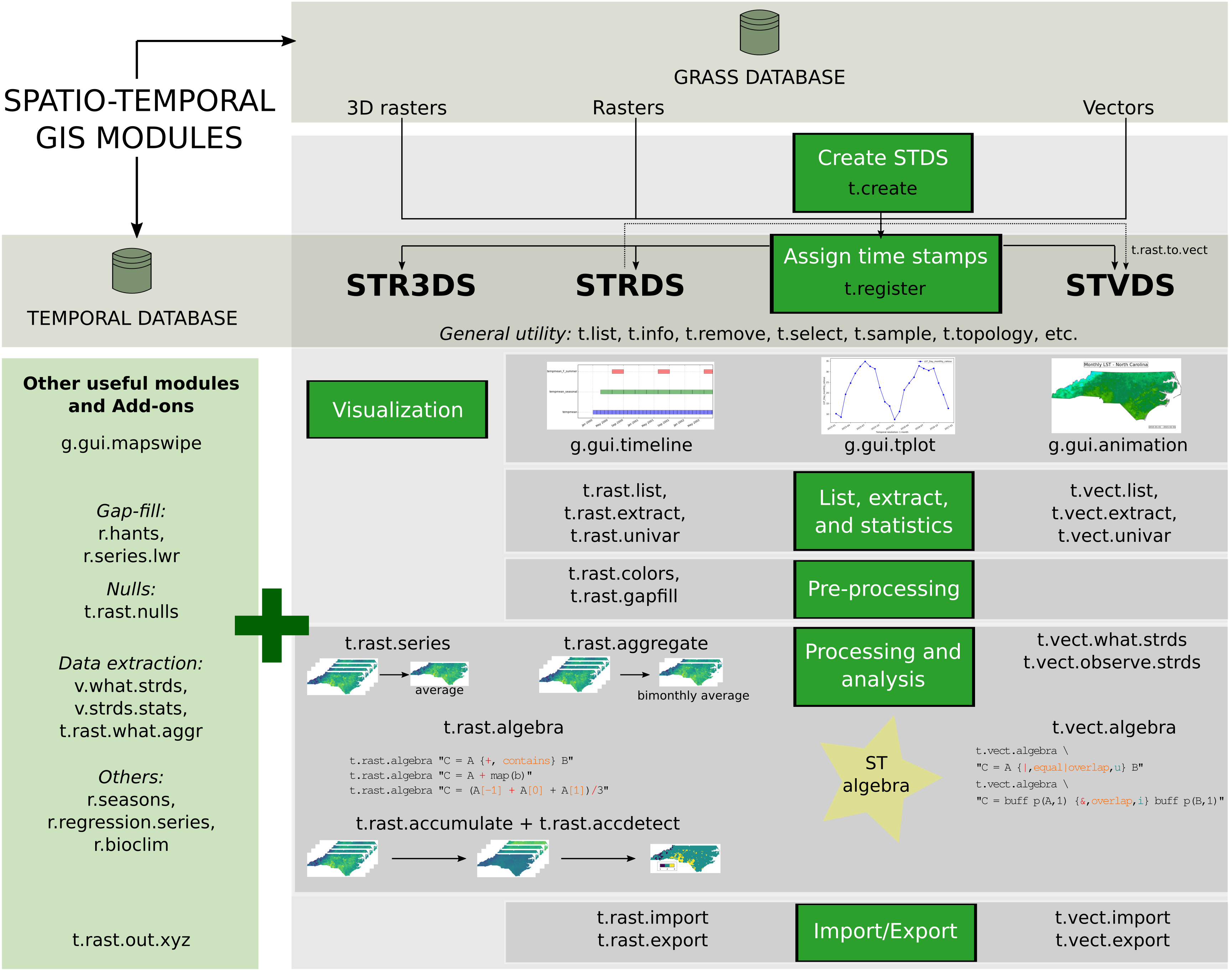{width=80%}# Manos a la obraEn esta segunda parte de la sesión vamos a recorrer los módulos temporales deGRASS GIS y demostrar su funcionalidad por medio de una serie de datos de temperatura de superficie (LST) de MODIS.Antes de empezar y para ganar tiempo, conectamos nuestro drive e instalamos GRASS en Google Colab.```{python}# import drive from google colabfrom google.colab import drive# mount drivedrive.mount("/content/drive")``````{python}%%bashDEBIAN_FRONTEND=noninteractive sudo add-apt-repository ppa:ubuntugis/ubuntugis-unstable apt update apt install grass subversion grass-devapt remove libproj22``````{python}!grass --config path```### Datos para la sesión- Producto MODIS: <ahref="https://lpdaac.usgs.gov/products/mod11b3v006/">MOD11B3 Collection 6</a>- Tile: h12v12- Composiciones mensuales - Resolución espacial: 5600m- Mapset *`modis_lst`* 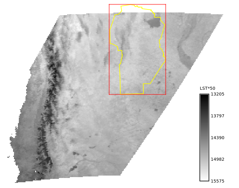{width=85%}### Iniciamos GRASSDefinimos las rutas y el mapset *`modis_lst`*```{python}import os# data directoryhomedir ="/content/drive/MyDrive/curso_grass_2023"# change to homedir so output files will be saved thereos.chdir(homedir)# GRASS GIS database variablesgrassdata = os.path.join(homedir, "grassdata")project ="posgar2007_4_cba"mapset ="modis_lst"``````{python}# import standard Python packages we needimport sysimport subprocess# ask GRASS GIS where its Python packages are to be able to run it from the notebooksys.path.append( subprocess.check_output(["grass", "--config", "python_path"], text=True).strip())```Importamos los paquetes de GRASS e iniciamos una sesión:```{python}# import the GRASS GIS packages we needimport grass.script as gsimport grass.jupyter as gj# Start the GRASS GIS Sessionsession = gj.init(grassdata, project, mapset)``````{python}# show current GRASS GIS settings, this also checks if the session worksgs.gisenv()```### Región computacional y máscaraListar los mapas raster y obtener información de uno de ellos```{python}# get list of raster maps in the 'modis_lst' mapsetlista_mapas = gs.list_grouped(type="raster")["modis_lst"]lista_mapas[:8]``````{python}# Get info from one of the raster mapsgs.raster_info(map="MOD11B3.A2015001.h12v12.single_LST_Day_6km")```Vamos a agregar el *semantic label* a cada mapa de LST```{python}# list only LST mapslista_lst = gs.list_grouped(type="raster", pattern="*LST_Day*")["modis_lst"]``````{python}# set semantic labelsfor i in lista_lst: gs.run_command("r.support",map=i, semantic_label="LST")``````{python}# Get info from one of the raster mapsgs.raster_info(map="MOD11B3.A2015001.h12v12.single_LST_Day_6km")["semantic_label"]```Establecemos la región computacional```{python}# set region to Cba boundaries with LST maps' resolutionprint(gs.read_command("g.region", vector="provincia_cba", align="MOD11B3.A2015001.h12v12.single_LST_Day_6km", flags="p"))```Aplicamos la máscara con los límites de la provincia de Córdoba```{python}# set a MASK to Cba boundarygs.run_command("r.mask", vector="provincia_cba")``````{python}# plotcba_map=gj.InteractiveMap(width =500, tiles="OpenStreetMap")cba_map.add_raster("MOD11B3.A2015001.h12v12.single_LST_Day_6km")cba_map.add_vector("provincia_cba")cba_map.add_layer_control(position ="bottomright")cba_map.show()```### Crear un conjunto de datos espacio-temporales (STDS)**[t.create](https://grass.osgeo.org/grass-stable/manuals/t.create.html)**- Crea una tabla SQLite en la base de datos temporal - Permite manejar grandes cantidades de mapas usando el STDS como entrada- Necesitamos especificar: - *tipo de mapas* (raster, raster3d o vector) - *tipo de tiempo* (absoluto o relativo)Creamos la STRDS```{python}# Create the STRDSgs.run_command("t.create",type="strds", temporaltype="absolute", output="LST_Day_monthly", title="Monthly LST Day 5.6 km", description="Monthly LST Day 5.6 km MOD11B3.006 Cordoba, 2015-2019")```Chequear si la STRDS fue creada```{python}# Check if the STRDS is createdgs.read_command("t.list",type="strds")```Obtener información sobre la STRDS```{python}# Get info about the STRDSprint(gs.read_command("t.info", input="LST_Day_monthly"))```### Registrar mapas en una STDS (asignar *timestamps*)**[t.register](https://grass.osgeo.org/grass-stable/manuals/t.register.html)**- Asigna o agrega timestamps a los mapas- Necesitamos: - el *STDS vacío* como entrada, i.e., la tabla SQLite contenedora, - la *lista de mapas* que se registrarán, - la *fecha de inicio*, - la opción de *incremento* junto con *-i* para la creación de intervalos ```{python}# Add time stamps to maps (i.e., register maps)gs.run_command("t.register",input="LST_Day_monthly", maps=lista_lst, start="2015-01-01", increment="1 months", flags="i")```Chequear la información sobre la STRDS nuevamente```{python}# Check info againprint(gs.read_command("t.info", input="LST_Day_monthly"))```Revisamos la lista de mapas en la STRDS```{python}# Check the list of maps in the STRDSprint(gs.read_command("t.rast.list", input="LST_Day_monthly"))```Chequeamos los valores mínimos y máximos de cada mapa```{python}# Check min and max per mapprint(gs.read_command("t.rast.list",input="LST_Day_monthly", columns="name,min,max"))```:::{.callout-note}Para más opciones sobre cómo registrar mapas, ver el manual de [t.register](https://grass.osgeo.org/grass-stable/manuals/t.register.html)y la wiki sobre [opciones para registrar mapas en STDS](https://grasswiki.osgeo.org/wiki/Temporal_data_processing/maps_registration).:::### Representación gráfica de STDSCrear una representación gráfica de la serie de tiempo```{python}!g.gui.timeline inputs=LST_Day_monthly```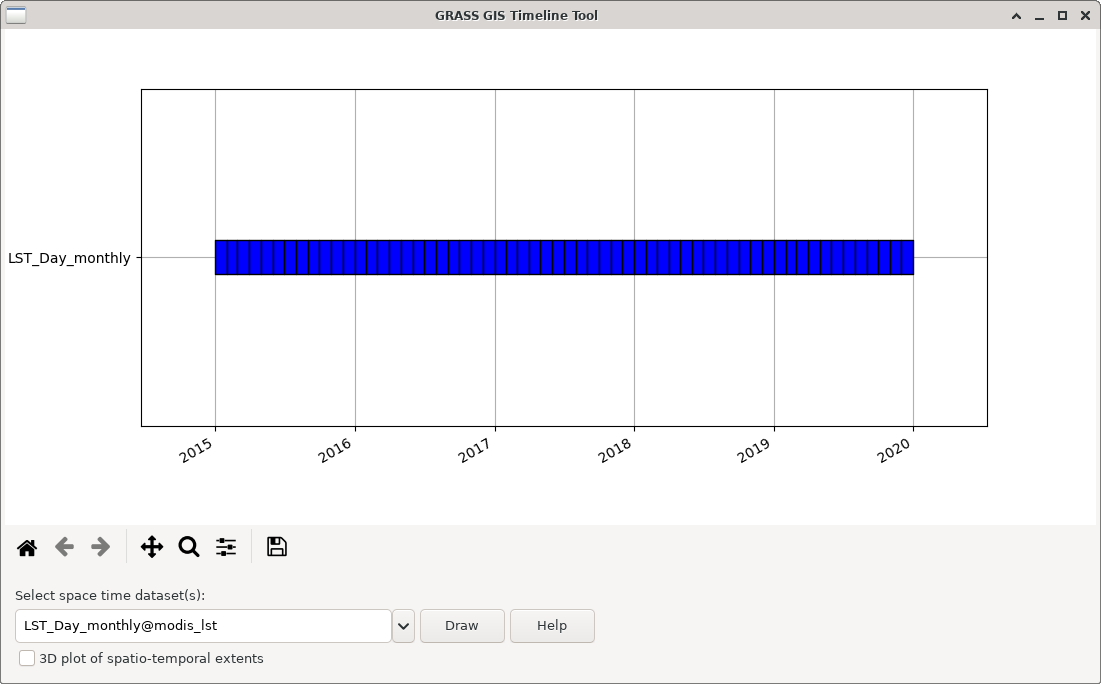{width=60%}:::{.callout-note}Ver el manual de <ahref="https://grass.osgeo.org/grass-stable/manuals/g.gui.timeline.html">g.gui.timeline</a> para más detalles.:::### Operaciones con álgebra temporal**[t.rast.algebra](https://grass.osgeo.org/grass-stable/manuals/t.rast.algebra.html)**- Realiza una amplia gama de operaciones de álgebra temporal y espacial basadas en la topología temporal de los mapas - Operadores temporales: unión, intersección, etc. - Funciones temporales: *start_time()*, *start_doy()*, etc. - Operadores espaciales (subconjunto de [r.mapcalc](https://grass.osgeo.org/grass-stable/manuals/r.mapcalc.html)) - Modificador de vecindario temporal: *[x,y,t]* - Otras funciones temporales como *t_snap()*, *buff_t()* o *t_shift()***¡pueden combinarse en expresiones complejas!**#### Desde K*50 a Celsius usando la calculadora temporalRe-escalar a grados Celsius```{python}# Re-scale data to degrees Celsiusexpression="LST_Day_monthly_celsius = LST_Day_monthly * 0.02 - 273.15"gs.run_command("t.rast.algebra", basename="LST_Day_monthly_celsius", suffix="gran", expression=expression)```Ver info de la nueva serie de tiempo```{python}# Check infoprint(gs.read_command("t.info", input="LST_Day_monthly_celsius"))```### Gráfico temporal: LST vs tiempoGráfico temporal de LST para la ciudad de Córdoba, Argentina```{python}# LST time series plot for Cba city center!g.gui.tplot strds=LST_Day_monthly_celsius coordinates=4323478.531282977,6541664.09350761 title="Monthly LST. City center of Cordoba" xlabel="Time" ylabel="LST"```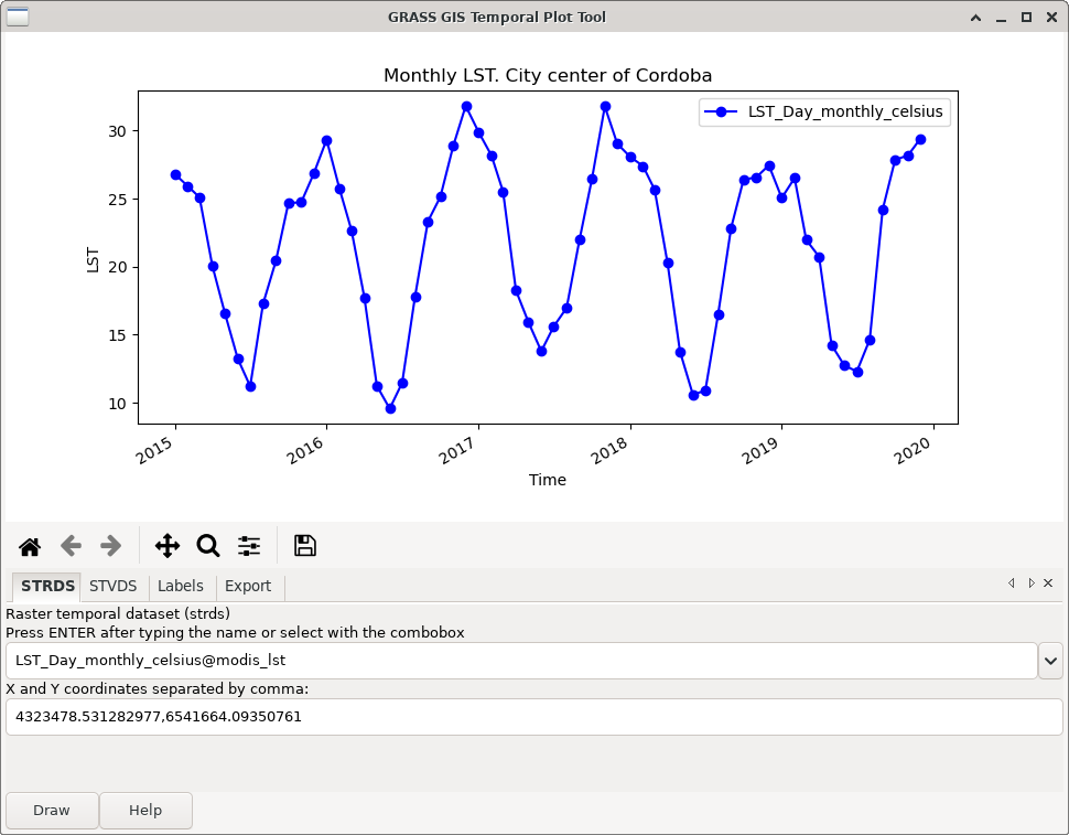{width=60%}En la interfaz de `g.gui.tplot`, las coordenadas del punto pueden ser escritasdirectamente, copiadas desde el mapa o seleccionadas interactivamente en el*map display*.:::{.callout-note}Para un único punto, ver <ahref="https://grass.osgeo.org/grass-stable/manuals/g.gui.tplot.html">g.gui.tplot</a>. Para un vector de puntos, ver <ahref="https://grass.osgeo.org/grass-stable/manuals/t.rast.what.html">t.rast.what</a>.:::### Listas y selecciones- **[t.list](https://grass.osgeo.org/grass-stable/manuals/t.list.html)** para listar las STDS y los mapas registrados en la base de datos temporal,- **[t.rast.list](https://grass.osgeo.org/grass-stable/manuals/t.rast.list.html)** para mapas en series temporales de rasters, y- **[t.vect.list](https://grass.osgeo.org/grass-stable/manuals/t.vect.list.html)** para mapas en series temporales de vectores.#### Variables usadas para hacer las listas y selecciones:::{style="background-color: rgba(200, 230, 255, 0.75);"}**STRDS:** *id, name, creator, mapset, temporal_type, creation_time, start_time, end_time, north, south, west, east, nsres, ewres, cols, rows, number_of_cells, min, max*::::::{style="background-color: rgba(200, 230, 255, 0.75);"}**STVDS:** *id, name, layer, creator, mapset, temporal_type, creation_time, start_time, end_time, north, south, west, east, points, lines, boundaries, centroids, faces, kernels, primitives, nodes, areas, islands, holes, volumes*:::#### Ejemplos de listas y seleccionesMapas cuyo valor mínimo es menor o igual a 10```{python}# Maps with minimum value lower than or equal to 10print(gs.read_command("t.rast.list",input="LST_Day_monthly_celsius", order="min", columns="name,start_time,min", where="min <= '10.0'"))```Mapas cuyo valor máximo es mayor a 30```{python}# Maps with maximum value higher than 30print(gs.read_command("t.rast.list",input="LST_Day_monthly_celsius", order="max", columns="name,start_time,max", where="max > '30.0'"))```Mapas contenidos entre dos fechas```{python}# Maps between two given datesprint(gs.read_command("t.rast.list",input="LST_Day_monthly_celsius", columns="name,start_time", where="start_time >= '2015-05' and start_time <= '2015-08-01 00:00:00'"))```Todos los mapas correspondientes al mes de Enero```{python}# Maps from Januaryprint(gs.read_command("t.rast.list",input="LST_Day_monthly_celsius", columns="name,start_time", where="strftime('%m', start_time)='01'"))```### Estadística descriptiva de STRDSImprimir estadísticas descriptivas univariadas para cada mapa dentro de la STRDS```{python}# Print univariate stats for maps within STRDSprint(gs.read_command("t.rast.univar",input="LST_Day_monthly_celsius"))```Obtener estadísticas extendidas con la opción -e y escribir la salida a unarchivo de texto```{python}# Write extended univariate stats output to a csv filegs.run_command("t.rast.univar", flags="e",input="LST_Day_monthly_celsius", output=os.path.join(homedir,"ext_stats_LST_Day_monthly_celsius.csv"), separator="comma")```Graficamos las series del promedio, mínimo y máximo por mapa:```{python}# Read the csv and plotimport pandas as pdlst = pd.read_csv(os.path.join(homedir,"ext_stats_LST_Day_monthly_celsius.csv"))lst['start'] = pd.to_datetime(lst.start, format="%Y-%m-%d", exact=False)lst.plot.line(1, [3,4,5], subplots=False)```### Agregación temporal 1: Serie completa**[t.rast.series](https://grass.osgeo.org/grass-stable/manuals/t.rast.series.html)**- Agrega STRDS *completas* o partes de ellas usando la opción *where*.- Diferentes métodos disponibles: promedio, mínimo, máximo, mediana, moda, etc.#### LST máxima y mínima del período 2015-2019Obtener los mapas de la máxima y mínima LST del período```{python}# Get maximum and minimum LST in the STRDSmethods=["maximum","minimum"]for m in methods: gs.run_command("t.rast.series",input="LST_Day_monthly_celsius", output=f"LST_Day_{m}", method=m)```Cambiar la paleta de colores a *celsius*```{python}# Change color pallete to celsiusgs.run_command("r.colors",map="LST_Day_minimum,LST_Day_maximum", color="celsius")```Graficamos los mapas obtenidos```{python}# Plotcba_map=gj.InteractiveMap(width =500, tiles="OpenStreetMap")cba_map.add_raster("LST_Day_minimum")cba_map.add_raster("LST_Day_maximum")cba_map.add_vector("provincia_cba")cba_map.add_layer_control(position ="bottomright")cba_map.show()```Usamos la calculadora de mapas temporal, `t.rast.mapcalc`,para obtener el mes de la LST mínima```{python}# Get month of maximum LSTexpression="if(LST_Day_monthly_celsius == LST_Day_minimum, start_month(), null())"gs.run_command("t.rast.mapcalc", flags="n", inputs="LST_Day_monthly_celsius", output="month_min_lst", expression=expression, basename="month_min_lst")```Obtener información del mapa resultante```{python}# Get basic infoprint(gs.read_command("t.info", input="month_min_lst"))```Obtenemos el primer mes en que aparece el mínimo de LST```{python}# Get the earliest month in which the maximum appeared (method minimum)gs.run_command("t.rast.series",input="month_min_lst", method="minimum", output="min_lst_date")```Remover la STRDS intermedia y los mapas que contiene:```{python}# Remove month_min_lst strds # we were only interested in the resulting aggregated mapgs.run_command("t.remove", flags="rfd", inputs="month_min_lst")```Chequeamos que la serie fue removida```{python}# check STRDS in our mapsetprint(gs.read_command("t.list"))```Mostrar el mapa resultante con la clase `Map` de `grass.jupyter````{python}# display resultsmm = gj.Map(width=450, use_region=True)mm.d_rast(map="min_lst_date")mm.d_vect(map="provincia_cba", type="boundary", color="#4D4D4D", width=2)mm.d_legend(raster="min_lst_date", title="Month", fontsize=10, at=(2,15,2,10))mm.d_barscale(length=50, units="kilometers", segment=4, fontsize=14, at=(73,7))mm.d_northarrow(at=(90,15))mm.d_text(text="Month of minimum LST", color="black", font="sans", size=4, bgcolor="white")mm.show()```:::{.callout-caution title="Tarea"}Podríamos haber hecho lo mismo pero anualmente para conocer en qué mes ocurre el máximo en cada año y así evaluar la ocurrencia de tendencias. Cómo lo harían?:::### Agregación temporal 2: granularidad**[t.rast.aggregate](https://grass.osgeo.org/grass-stable/manuals/t.rast.aggregate.html)**- Agrega mapas raster dentro de STRDS con diferentes **granularidades** - La opción *where* permite establecer fechas específicas para la agregación- Diferentes métodos disponibles: promedio, mínimo, máximo, mediana, moda, etc.#### De LST mensual a estacionalLST media estacional```{python}# 3-month mean LSTgs.run_command("t.rast.aggregate",input="LST_Day_monthly_celsius", output="LST_Day_mean_3month", basename="LST_Day_mean_3month", suffix="gran", method="average", granularity="3 months")```Chequear info```{python}# Check infoprint(gs.read_command("t.info",input="LST_Day_mean_3month"))```Chequear lista de mapas```{python}# Check map listprint(gs.read_command("t.rast.list",input="LST_Day_mean_3month"))```Establecer la paleta de colores *celsius* para la STRDS estacional```{python}# Set STRDS color table to celsius degreesgs.run_command("t.rast.colors",input="LST_Day_mean_3month", color="celsius")```Mostramos la serie recientemente creada con una animación. Para eso vamosa usar la clase `TimeSeriesMap` de `grass.jupyter````{python}## Display newly created NDVI time series maplstseries = gj.TimeSeriesMap(use_region=True)lstseries.add_raster_series("LST_Day_mean_3month", fill_gaps=False)lstseries.d_legend(color="black", at=(10,40,2,6))lstseries.show() # Create TimeSlider# optionally, write out to animated GIFlstseries.save("lstseries.gif")```:::{.callout-warning title="Tarea"}Ahora que ya conocen[t.rast.aggregate](https://grass.osgeo.org/grass-stable/manuals/t.rast.aggregate.html), extraigan el mes de máximo LST por año y luego vean si hay alguna tendenciapositiva o negativa, es decir, si los valores máximos de LST se observan más tarde o más temprano con el tiempo (años).Una solución podría ser...```{python}gs.run_command("t.rast.aggregate",input="LST_Day_monthly_celsius", output="month_max_LST_per_year", basename="month_max_LST", suffix="gran", method="max_raster", granularity="1 year")gs.run_command("t.rast.series", input="month_max_LST_per_year", output="slope_month_max_LST", method="slope")```:::### Agregación vs Climatología:::: columns:::{.column width="50%"}::::::{.column width="50%"}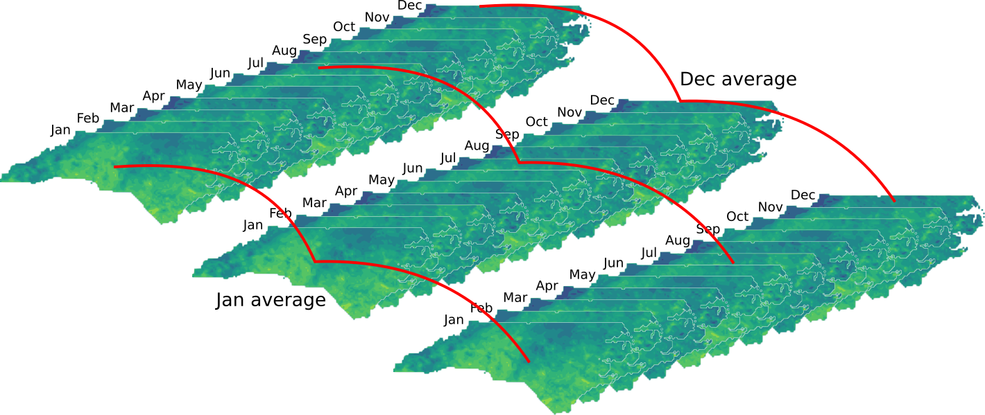:::::::#### Climatologías mensualesLST promedio de Enero```{python}# January average LSTgs.run_command("t.rast.series",input="LST_Day_monthly_celsius", method="average", where="strftime('%m', start_time)='01'", output="LST_average_jan")```Climatología para todos los meses```{python}# for all monthsmonths=['{0:02d}'.format(m) for m inrange(1,13)]methods=["average"]for m in months:for me in methods: gs.run_command("t.rast.series", input="LST_Day_monthly_celsius", method=me, where=f"strftime('%m', start_time)='{m}'", output=f"LST_{me}_{m}")```:::{.callout-warning title="Tarea"}- Comparar las medias mensuales con las climatologías mensuales- Las climatologías que creamos forman una STRDS?:::### Anomalías anualesSe necesitan:- promedio y desviación estándar general de la serie- promedios anuales$$AnomaliaStd_i = \frac{Media_i - Media}{SD}$$Obtenemos primero el promedio y el desvío estándar general de la serie```{python}# Get general average and SDmethods=["average","stddev"]for me in methods: gs.run_command("t.rast.series",input="LST_Day_monthly_celsius", method=me, output=f"LST_Day_{me}")```y luego los promedios anuales```{python}# Get annual averagesgs.run_command("t.rast.aggregate",input="LST_Day_monthly_celsius", method="average", granularity="1 years", output="LST_yearly_average", basename="LST_yearly_average")```Utilizamos el álgebra temporal para estimar las anomalías anuales```{python}# Estimate annual anomaliesexpression="LST_year_anomaly = (LST_yearly_average - map(LST_Day_average)) / map(LST_Day_stddev)"gs.run_command("t.rast.algebra", basename="LST_year_anomaly", expression=expression)```Establecer la paleta de colores *differences* para toda la serie (esto permite tomar el minimo y maximo general de la serie)```{python}# Set difference color tablegs.run_command("t.rast.colors",input="LST_year_anomaly", color="difference")```Mostramos los resultados con una animación```{python}# Animation of annual anomaliesanomalies = gj.TimeSeriesMap(use_region=True)anomalies.add_raster_series("LST_year_anomaly", fill_gaps=False)anomalies.d_legend(color="black", at=(10,40,2,6))anomalies.show()```### Isla de calor superficial urbana (Surface Urban Heat Island - SUHI)- La temperatura del aire de una zona urbana es más alta que la de las zonas cercanas- La UHI tiene efectos negativos en la calidad del agua y el aire, la biodiversidad, la salud humana y el clima.- La SUHI también está muy relacionada con la salud, ya que influye en la UHI {width=60%}### Estadística zonal en series de tiempo de datos raster**[v.strds.stats](https://grass.osgeo.org/grass7/manuals/addons/v.strds.stats.html)**- Permite obtener datos de series de tiempo agregados espacialmente para polígonos de un mapa vectorial#### SUHI estival para *Córdoba* y alrededoresInstalar la extensión *v.strds.stats*```{python}# Install v.strds.stats add-ongs.run_command("g.extension", extension="v.strds.stats")```Listar mapas```{python}# List maps in seasonal time seriesprint(gs.run_command("t.rast.list",input="LST_Day_mean_3month"))```Extraer LST promedio de verano para el Gran Córdoba```{python}# Extract summer average LST for Cba urban areags.run_command("v.strds.stats",input="area_edificada_cba", strds="LST_Day_mean_3month", where="fna == 'Gran Córdoba'", t_where="strftime('%m', start_time)='02'", output="cba_summer_lst", method="average")```Crear buffer externo - 30 km```{python}# Create outside buffer - 30 kmgs.run_command("v.buffer",input="cba_summer_lst", distance=30000, output="cba_summer_lst_buf30")```Crear buffer interno - 15 km```{python}# Create inside buffer - 15 kmgs.run_command("v.buffer",input="cba_summer_lst", distance=15000, output="cba_summer_lst_buf15")```Remover el área del buffer 15 km del buffer de 30 km```{python}# Remove 15km buffer area from the 30km buffer areags.run_command("v.overlay", ainput="cba_summer_lst_buf15", binput="cba_summer_lst_buf30", operator="xor", output="cba_surr")```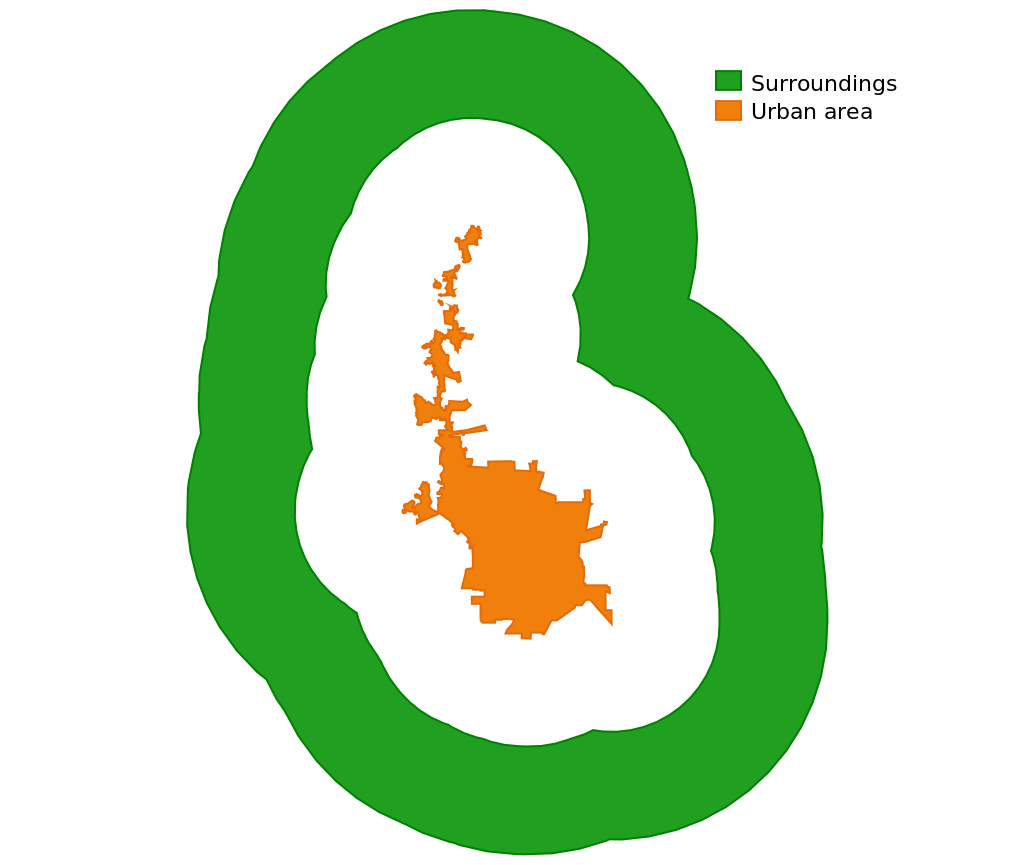{width=50%}Extraer estadísticas para los alrededores del Gran Córdoba```{python}# Extract zonal stats for Cba surroundingsgs.run_command("v.strds.stats",input="cba_surr", strds="LST_Day_mean_3month", t_where="strftime('%m', start_time)='02'", method="average", output="cba_surr_summer_lst")```Chequear la LST estival promedio para el Gran Córdoba y alrededores```{python}# Take a look at mean summer LST in Cba and surroundingsgs.vector_db_select("cba_summer_lst")["values"]``````{python}gs.vector_db_select("cba_surr_summer_lst")["values"]``````{python}tabla1 = pd.DataFrame.from_dict(gs.vector_db_select(map="cba_summer_lst")['values'], orient='index', columns=gs.vector_db_select(map="cba_summer_lst")['columns'])tabla1``````{python}# crear un data frame a partir del vectortabla2 = pd.DataFrame.from_dict(gs.vector_db_select(map="cba_surr_summer_lst")['values'], orient='index', columns=gs.vector_db_select(map="cba_surr_summer_lst")['columns'])tabla2``````{python}# table massagingdf1 = tabla1.loc[1:,['cat', 'LST_Day_mean_3month_2015_02_01_average', 'LST_Day_mean_3month_2016_02_01_average', 'LST_Day_mean_3month_2017_02_01_average', 'LST_Day_mean_3month_2018_02_01_average', 'LST_Day_mean_3month_2019_02_01_average']]df2 = tabla2.loc[1:,['cat', 'LST_Day_mean_3month_2015_02_01_average', 'LST_Day_mean_3month_2016_02_01_average', 'LST_Day_mean_3month_2017_02_01_average', 'LST_Day_mean_3month_2018_02_01_average', 'LST_Day_mean_3month_2019_02_01_average']]``````{python}tables = [df1,df2]suhi = pd.concat(tables)suhi['cat'] = suhi.indexsuhi``````{python}suhi_long = suhi.melt(id_vars="cat", var_name="date", value_name="LST_Day_mean_3month_average")suhi_long```:::{.callout-warning title="Tarea"}Se animan a hacer un gráfico de barras con librerías de Python para representar los valores promedios por año para la zona urbana y alrededores?:::```{python}import matplotlib.pyplot as pltimport seaborn as snsimport numpy as npsuhi_long['setting'] = np.where(suhi_long['cat']==1, 'Non Urban', 'Urban')``````{python}plt.figure(figsize=(10, 10))g = sns.barplot(data= suhi_long, x="date", y="LST_Day_mean_3month_average", hue="setting")g.set_xticklabels(["2015", "2016", "2017", "2018", "2019"])plt.xlabel("Year")plt.ylabel("LST Day mean 3month average")sns.move_legend(g, "upper right", title="Setting")plt.show()```# Recursos (muy) útiles - [Temporal data processing wiki](https://grasswiki.osgeo.org/wiki/Temporal_data_processing)- [GRASS GIS and R for time series processing wiki](https://grasswiki.osgeo.org/wiki/Temporal_data_processing/GRASS_R_raster_time_series_processing)- [GRASS GIS temporal workshop at NCSU](http://ncsu-geoforall-lab.github.io/grass-temporal-workshop/)- [GRASS GIS course IRSAE 2018](http://training.gismentors.eu/grass-gis-irsae-winter-course-2018/index.html)- [GRASS GIS workshop held in Jena 2023](https://training.gismentors.eu/grass-gis-workshop-jena/)- [Using Satellite Data for Species Distribution Modeling with GRASS GIS and R](https://veroandreo.github.io/grass_ncsu_2023/studio_index.html). Workshop en NCSU. Abril, 2023.# Referencias::: {#refs .tiny}:::


